Source: NVIDIA PTX ISA 9.4 documentation.
While the specific resources available in a given target GPU will vary, the kinds of resources will be common across platforms, and these resources are abstracted in PTX through state spaces and data types.
5.1. State Spaces#
A state space is a storage area with particular characteristics. All variables reside in some state space. The characteristics of a state space include its size, addressability, access speed, access rights, and level of sharing between threads.
The state spaces defined in PTX are a byproduct of parallel programming and graphics programming. The list of state spaces is shown in Table 6,and properties of state spaces are shown in Table 7.
Name |
Description |
|---|---|
|
Registers, fast. |
|
Special registers. Read-only; pre-defined; platform-specific. |
|
Shared, read-only memory. |
|
Global memory, shared by all threads. |
|
Local memory, private to each thread. |
|
Kernel parameters, defined per-grid; or Function or local parameters, defined per-thread. |
|
Addressable memory, defined per CTA, accessible to all threads in the cluster throughout the lifetime of the CTA that defines it. |
|
Global texture memory (deprecated). |
Name |
Addressable |
Initializable |
Access |
Sharing |
|---|---|---|---|---|
|
No |
No |
R/W |
per-thread |
|
No |
No |
RO |
per-CTA |
|
Yes |
Yes1 |
RO |
per-grid |
|
Yes |
Yes1 |
R/W |
Context |
|
Yes |
No |
R/W |
per-thread |
|
Yes2 |
No |
RO |
per-grid |
|
Restricted3 |
No |
R/W |
per-thread |
|
Yes |
No |
R/W |
per-cluster5 |
|
No4 |
Yes, via driver |
RO |
Context |
|
Notes: 1 Variables in 2 Accessible only via the 3 Accessible via 4 Accessible only via the 5 Visible to the owning CTA and other active CTAs in the cluster. |
||||
5.1.1. Register State Space#
Registers (.reg state space) are fast storage locations. The number of registers is limited, and
will vary from platform to platform. When the limit is exceeded, register variables will be spilled
to memory, causing changes in performance. For each architecture, there is a recommended maximum
number of registers to use (see the CUDA Programming Guide for details).
Registers may be typed (signed integer, unsigned integer, floating point, predicate) or
untyped. Register size is restricted; aside from predicate registers which are 1-bit, scalar
registers have a width of 8-, 16-, 32-, 64-, or 128-bits, and vector registers have a width of
16-, 32-, 64-, or 128-bits. The most common use of 8-bit registers is with ld, st, and cvt
instructions, or as elements of vector tuples.
Registers differ from the other state spaces in that they are not fully addressable, i.e., it is not
possible to refer to the address of a register. When compiling to use the Application Binary
Interface (ABI), register variables are restricted to function scope and may not be declared at
module scope. When compiling legacy PTX code (ISA versions prior to 3.0) containing module-scoped
.reg variables, the compiler silently disables use of the ABI. Registers may have alignment
boundaries required by multi-word loads and stores.
5.1.2. Special Register State Space#
The special register (.sreg) state space holds predefined, platform-specific registers, such as
grid, cluster, CTA, and thread parameters, clock counters, and performance monitoring registers. All
special registers are predefined.
5.1.3. Constant State Space#
The constant (.const) state space is a read-only memory initialized by the host. Constant memory
is accessed with a ld.const instruction. Constant memory is restricted in size, currently
limited to 64 KB which can be used to hold statically-sized constant variables. There is an
additional 640 KB of constant memory, organized as ten independent 64 KB regions. The driver may
allocate and initialize constant buffers in these regions and pass pointers to the buffers as kernel
function parameters. Since the ten regions are not contiguous, the driver must ensure that constant
buffers are allocated so that each buffer fits entirely within a 64 KB region and does not span a
region boundary.
Statically-sized constant variables have an optional variable initializer; constant variables with no explicit initializer are initialized to zero by default. Constant buffers allocated by the driver are initialized by the host, and pointers to such buffers are passed to the kernel as parameters. See the description of kernel parameter attributes in Kernel Function Parameter Attributes for more details on passing pointers to constant buffers as kernel parameters.
5.1.3.1. Banked Constant State Space (deprecated)#
Previous versions of PTX exposed constant memory as a set of eleven 64 KB banks, with explicit bank numbers required for variable declaration and during access.
Prior to PTX ISA version 2.2, the constant memory was organized into fixed size banks. There were
eleven 64 KB banks, and banks were specified using the .const[bank] modifier, where bank
ranged from 0 to 10. If no bank number was given, bank zero was assumed.
By convention, bank zero was used for all statically-sized constant variables. The remaining banks were used to declare incomplete constant arrays (as in C, for example), where the size is not known at compile time. For example, the declaration
.extern .const[2] .b32 const_buffer[];
resulted in const_buffer pointing to the start of constant bank two. This pointer could then be
used to access the entire 64 KB constant bank. Multiple incomplete array variables declared in the
same bank were aliased, with each pointing to the start address of the specified constant bank.
To access data in constant banks 1 through 10, the bank number was required in the state space of the load instruction. For example, an incomplete array in bank 2 was accessed as follows:
.extern .const[2] .b32 const_buffer[];
ld.const[2].b32  %r1, [const_buffer+4]; // load second word
In PTX ISA version 2.2, we eliminated explicit banks and replaced the incomplete array representation of driver-allocated constant buffers with kernel parameter attributes that allow pointers to constant buffers to be passed as kernel parameters.
5.1.4. Global State Space#
The global (.global) state space is memory that is accessible by all threads in a context. It is
the mechanism by which threads in different CTAs, clusters, and grids can communicate. Use
ld.global, st.global, and atom.global to access global variables.
Global variables have an optional variable initializer; global variables with no explicit initializer are initialized to zero by default.
5.1.5. Local State Space#
The local state space (.local) is private memory for each thread to keep its own data. It is
typically standard memory with cache. The size is limited, as it must be allocated on a per-thread
basis. Use ld.local and st.local to access local variables.
When compiling to use the Application Binary Interface (ABI), .local state-space variables
must be declared within function scope and are allocated on the stack. In implementations that do
not support a stack, all local memory variables are stored at fixed addresses, recursive function
calls are not supported, and .local variables may be declared at module scope. When compiling
legacy PTX code (ISA versions prior to 3.0) containing module-scoped .local variables, the
compiler silently disables use of the ABI.
5.1.6. Parameter State Space#
The parameter (.param) state space is used (1) to pass input arguments from the host to the
kernel, (2a) to declare formal input and return parameters for device functions called from within
kernel execution, and (2b) to declare locally-scoped byte array variables that serve as function
call arguments, typically for passing large structures by value to a function. Kernel function
parameters differ from device function parameters in terms of access and sharing (read-only versus
read-write, per-kernel versus per-thread). Note that PTX ISA versions 1.x supports only kernel
function parameters in .param space; device function parameters were previously restricted to the
register state space. The use of parameter state space for device function parameters was introduced
in PTX ISA version 2.0 and requires target architecture sm_20 or higher. Additional sub-qualifiers
::entry or ::func can be specified on instructions with .param state space to indicate
whether the address refers to kernel function parameter or device function parameter. If no
sub-qualifier is specified with the .param state space, then the default sub-qualifier is specific
to and dependent on the exact instruction. For example, st.param is equivalent to st.param::func
whereas isspacep.param is equivalent to isspacep.param::entry. Refer to the instruction
description for more details on default sub-qualifier assumption.
Note
The location of parameter space is implementation specific. For example, in some implementations
kernel parameters reside in global memory. No access protection is provided between parameter and
global space in this case. Though the exact location of the kernel parameter space is
implementation specific, the kernel parameter space window is always contained within the global
space window. Similarly, function parameters are mapped to parameter passing registers and/or
stack locations based on the function calling conventions of the Application Binary Interface
(ABI). Therefore, PTX code should make no assumptions about the relative locations or ordering
of .param space variables.
5.1.6.1. Kernel Function Parameters#
Each kernel function definition includes an optional list of parameters. These parameters are
addressable, read-only variables declared in the .param state space. Values passed from the host
to the kernel are accessed through these parameter variables using ld.param instructions. The
kernel parameter variables are shared across all CTAs from all clusters within a grid.
The address of a kernel parameter may be moved into a register using the mov instruction. The
resulting address is in the .param state space and is accessed using ld.param instructions.
Example
.entry foo ( .param .b32 N, .param .align 8 .b8 buffer[64] )
{
.reg .u32 %n;
.reg .f64 %d;
ld.param.u32 %n, [N];
ld.param.f64 %d, [buffer];
...
plaintext
Example
.entry bar ( .param .b32 len )
{
.reg .u32 %ptr, %n;
mov.u32 %ptr, len;
ld.param.u32 %n, [%ptr];
...
plaintext
Kernel function parameters may represent normal data values, or they may hold addresses to objects in constant, global, local, or shared state spaces. In the case of pointers, the compiler and runtime system need information about which parameters are pointers, and to which state space they point. Kernel parameter attribute directives are used to provide this information at the PTX level. See Kernel Function Parameter Attributes for a description of kernel parameter attribute directives.
Note
The current implementation does not allow creation of generic pointers to constant variables
(cvta.const) in programs that have pointers to constant buffers passed as kernel parameters.
5.1.6.2. Kernel Function Parameter Attributes#
Kernel function parameters may be declared with an optional .ptr attribute to indicate that a
parameter is a pointer to memory, and also indicate the state space and alignment of the memory
being pointed to. Kernel Parameter Attribute: .ptr
describes the .ptr kernel parameter attribute.
5.1.6.3. Kernel Parameter Attribute: .ptr#
.ptr
Kernel parameter alignment attribute.
Syntax
.param .type .ptr .space .align N  varname
.param .type .ptr        .align N  varname
.space = { .const, .global, .local, .shared };
Description
Used to specify the state space and, optionally, the alignment of memory pointed to by a pointer type kernel parameter. The alignment value N, if present, must be a power of two. If no state space is specified, the pointer is assumed to be a generic address pointing to one of const, global, local, or shared memory. If no alignment is specified, the memory pointed to is assumed to be aligned to a 4 byte boundary.
Spaces between .ptr, .space, and .align may be eliminated to improve readability.
Examples
.entry foo ( .param .u32 param1,
             .param .u32 .ptr.global.align 16 param2,
             .param .u32 .ptr.const.align 8 param3,
             .param .u32 .ptr.align 16 param4  // generic address
                                               // pointer
) { .. }
5.1.6.4. Device Function Parameters#
PTX ISA version 2.0 extended the use of parameter space to device function parameters. The most
common use is for passing objects by value that do not fit within a PTX register, such as C
structures larger than 8 bytes. In this case, a byte array in parameter space is used. Typically,
the caller will declare a locally-scoped .param byte array variable that represents a flattened
C structure or union. This will be passed by value to a callee, which declares a .param formal
parameter having the same size and alignment as the passed argument.
Example
// pass object of type struct { double d; int y; };
.func foo ( .reg .b32 N, .param .align 8 .b8 buffer[12] )
{
.reg .f64 %d;
.reg .s32 %y;
ld.param.f64 %d, [buffer];
ld.param.s32 %y, [buffer+8];
...
plaintext
}
// code snippet from the caller
// struct { double d; int y; } mystruct; is flattened, passed to foo
…
.reg .f64 dbl;
.reg .s32 x;
.param .align 8 .b8 mystruct;
…
st.param.f64 [mystruct+0], dbl;
st.param.s32 [mystruct+8], x;
call foo, (4, mystruct);
…
See the section on function call syntax for more details.
Function input parameters may be read via ld.param and function return parameters may be written
using st.param; it is illegal to write to an input parameter or read from a return parameter.
Aside from passing structures by value, .param space is also required whenever a formal
parameter has its address taken within the called function. In PTX, the address of a function input
parameter may be moved into a register using the mov instruction. Note that the parameter will
be copied to the stack if necessary, and so the address will be in the .local state space and is
accessed via ld.local and st.local instructions. It is not possible to use mov to get
the address of or a locally-scoped .param space variable. Starting PTX ISA version 6.0, it is
possible to use mov instruction to get address of return parameter of device function.
Example
// pass array of up to eight floating-point values in buffer
.func foo ( .param .b32 N, .param .b32 buffer[32] )
{
.reg .u32 %n, %r;
.reg .f32 %f;
.reg .pred %p;
ld.param.u32 %n, [N];
mov.u32 %r, buffer; // forces buffer to .local state space
plaintext
Loop:
setp.eq.u32 %p, %n, 0;
@%p bra Done;
ld.local.f32 %f, [%r];
…
add.u32 %r, %r, 4;
sub.u32 %n, %n, 1;
bra Loop;
Done:
…
}
5.1.7. Shared State Space#
The shared (.shared) state space is a memory that is owned by an executing CTA and is accessible
to the threads of all the CTAs within a cluster. An address in shared memory can be read and written
by any thread in a CTA cluster.
Additional sub-qualifiers ::cta or ::cluster can be specified on instructions with
.shared state space to indicate whether the address belongs to the shared memory window of the
executing CTA or of any CTA in the cluster respectively. The addresses in the .shared::cta
window also fall within the .shared::cluster window. If no sub-qualifier is specified with the
.shared state space, then it defaults to ::cta. For example, ld.shared is equivalent to
ld.shared::cta.
Variables declared in .shared state space refer to the memory addresses in the current
CTA. Instruction mapa gives the .shared::cluster address of the corresponding variable in
another CTA in the cluster.
Shared memory typically has some optimizations to support the sharing. One example is broadcast; where all threads read from the same address. Another is sequential access from sequential threads.
Maximum capacity for statically allocated shared memory is 48 KB per CTA.
Architecture specific targets such as sm_90a, support extended statically allocated shared memory
capacity beyond 48 KB per CTA as described below:
Target architecture |
Maximum statically allocated shared memory size |
|---|---|
|
228 KB |
|
228 KB |
|
228 KB |
|
100 KB |
5.1.8. Texture State Space (deprecated)#
The texture (.tex) state space is global memory accessed via the texture instruction. It is
shared by all threads in a context. Texture memory is read-only and cached, so accesses to texture
memory are not coherent with global memory stores to the texture image.
The GPU hardware has a fixed number of texture bindings that can be accessed within a single kernel
(typically 128). The .tex directive will bind the named texture memory variable to a hardware
texture identifier, where texture identifiers are allocated sequentially beginning with
zero. Multiple names may be bound to the same physical texture identifier. An error is generated if
the maximum number of physical resources is exceeded. The texture name must be of type .u32 or
.u64.
Physical texture resources are allocated on a per-kernel granularity, and .tex variables are
required to be defined in the global scope.
Texture memory is read-only. A texture’s base address is assumed to be aligned to a 16 byte boundary.
Example
.tex .u32 tex_a;         // bound to physical texture 0
.tex .u32 tex_c, tex_d;  // both bound to physical texture 1
.tex .u32 tex_d;         // bound to physical texture 2
.tex .u32 tex_f;         // bound to physical texture 3
Note
Explicit declarations of variables in the texture state space is deprecated, and programs should
instead reference texture memory through variables of type .texref. The .tex directive is
retained for backward compatibility, and variables declared in the .tex state space are
equivalent to module-scoped .texref variables in the .global state space.
For example, a legacy PTX definitions such as
.tex .u32 tex_a;
is equivalent to:
.global .texref tex_a;
See Texture Sampler and Surface Types for the
description of the .texref type and Texture Instructions
for its use in texture instructions.
5.2. Types#
5.2.1. Fundamental Types#
In PTX, the fundamental types reflect the native data types supported by the target architectures. A fundamental type specifies both a basic type and a size. Register variables are always of a fundamental type, and instructions operate on these types. The same type-size specifiers are used for both variable definitions and for typing instructions, so their names are intentionally short.
Table 8 lists the fundamental type specifiers for each basic type:
Basic Type |
Fundamental Type Specifiers |
|---|---|
Signed integer |
|
Unsigned integer |
|
Floating-point |
|
Bits (untyped) |
|
Predicate |
|
Most instructions have one or more type specifiers, needed to fully specify instruction behavior. Operand types and sizes are checked against instruction types for compatibility.
Two fundamental types are compatible if they have the same basic type and are the same size. Signed and unsigned integer types are compatible if they have the same size. The bit-size type is compatible with any fundamental type having the same size.
In principle, all variables (aside from predicates) could be declared using only bit-size types, but typed variables enhance program readability and allow for better operand type checking.
5.2.2. Restricted Use of Sub-Word Sizes#
The .u8, .s8, and .b8 instruction types are restricted to ld, st, add, sub,
min, max, neg and cvt instructions. The .f16 floating-point type is allowed
in half precision floating point instructions and texture fetch instructions.
The .f16x2 floating point type is allowed only in half precision
floating point arithmetic instructions and texture fetch instructions.
For convenience, ld, st, and cvt instructions permit source and destination data
operands to be wider than the instruction-type size, so that narrow values may be loaded, stored,
and converted using regular-width registers. For example, 8-bit or 16-bit values may be held
directly in 32-bit or 64-bit registers when being loaded, stored, or converted to other types and
sizes.
5.2.3. Alternate Floating-Point Data Formats#
The fundamental floating-point types supported in PTX have implicit bit representations that
indicate the number of bits used to store exponent and mantissa. For example, the .f16 type
indicates 5 bits reserved for exponent and 10 bits reserved for mantissa. In addition to the
floating-point representations assumed by the fundamental types, PTX allows the following alternate
floating-point data formats:
-
bf16data format: -
This data format is a 16-bit floating point format with 8 bits for exponent and 7 bits for mantissa. A register variable containing
bf16data must be declared with.b16type. -
e4m3data format: -
This data format is an 8-bit floating point format with 4 bits for exponent and 3 bits for mantissa. The
e4m3encoding does not support infinity andNaNvalues are limited to0x7fand0xff. A register variable containinge4m3value must be declared using bit-size type. -
e5m2data format: -
This data format is an 8-bit floating point format with 5 bits for exponent and 2 bits for mantissa. A register variable containing
e5m2value must be declared using bit-size type. -
tf32data format: -
This data format is a special 32-bit floating point format supported by the matrix multiply-and-accumulate instructions, with the same range as
.f32and reduced precision (>=10 bits). The internal layout oftf32format is implementation defined. PTX facilitates conversion from single precision.f32type totf32format. A register variable containingtf32data must be declared with.b32type. -
e2m1data format: -
This data format is a 4-bit floating point format with 2 bits for exponent and 1 bit for mantissa. The
e2m1encoding does not support infinity andNaN.e2m1values must be used in a packed format specified ase2m1x2. A register variable containing twoe2m1values must be declared with.b8type. -
e2m3data format: -
This data format is a 6-bit floating point format with 2 bits for exponent and 3 bits for mantissa. The
e2m3encoding does not support infinity andNaN.e2m3values must be used in a packed format specified ase2m3x2. A register variable containing twoe2m3values must be declared with.b16type where each.b8element has 6-bit floating point value and 2 MSB bits padded with zeros. -
e3m2data format: -
This data format is a 6-bit floating point format with 3 bits for exponent and 2 bits for mantissa. The
e3m2encoding does not support infinity andNaN.e3m2values must be used in a packed format specified ase3m2x2. A register variable containing twoe3m2values must be declared with.b16type where each.b8element has 6-bit floating point value and 2 MSB bits padded with zeros. -
ue8m0data format: -
This data format is an 8-bit unsigned floating-point format with 8 bits for exponent and 0 bits for mantissa. The
ue8m0encoding does not support infinity.NaNvalue is limited to0xff.ue8m0values must be used in a packed format specified asue8m0x2. A register variable containing twoue8m0values must be declared with.b16type. -
ue4m3data format: -
This data format is a 7-bit unsigned floating-point format with 4 bits for exponent and 3 bits for mantissa. The
ue4m3encoding does not support infinity.NaNvalue is limited to0x7f. A register variable containing singleue4m3value must be declared with.b8type having MSB bit padded with zero. -
ue5m3data format: -
This data format is a 8-bit unsigned floating-point format with 5 bits for exponent and 3 bits for mantissa. The
ue5m3encoding does not support infinity.NaNvalue is limited to0xff. A register variable containing singleue5m3value must be declared with.b8type.
Alternate data formats cannot be used as fundamental types. They are supported as source or destination formats by certain instructions.
5.2.4. Fixed-point Data format#
PTX supports following fixed-point data formats:
-
s2f6data format: -
This data format is 8-bit signed 2’s complement integer with 2 sign-integer bits and 6 fractional bits with form xx.xxxxxx. The
s2f6encoding does not support infinity andNaN.s2f6value = s8 value * 2^(-6) Positive max representation = 01.111111 = 127 * 2^(-6) = 1.984375 Negative max representation = 10.000000 = -128 * 2^(-6) = -2.0
5.2.5. Packed Data Types#
Certain PTX instructions operate on two or more sets of inputs in parallel, and produce two or more sets of outputs. Such instructions can use the data stored in a packed format. PTX supports either two or four values of the same scalar data type to be packed into a single, larger value. The packed value is considered as a value of a packed data type. In this section we describe the packed data types supported in PTX.
5.2.5.1. Packed Floating Point Data Types#
PTX supports various variants of packed floating point data types. Out of them, only .f16x2 is
supported as a fundamental type, while others cannot be used as fundamental types - they are
supported as instruction types on certain instructions. When using an instruction with such
non-fundamental types, the operand data variables must be of bit type of appropriate size.
For example, all of the operand variables must be of type .b32 for an instruction with
instruction type as .bf16x2.
Table 9 described various variants
of packed floating point data types in PTX.
Packed floating point type |
Number of elements contained in a packed format |
Type of each element |
Register variable type to be used in the declaration |
|---|---|---|---|
|
Two |
|
|
|
|
|
|
|
|
|
|
|
|
|
|
|
|
||
|
|
||
|
|
||
|
|
||
|
|
||
|
|
||
|
|
|
|
|
Four |
|
|
|
|
||
|
|
||
|
|
||
|
|
||
|
|
||
|
|
|
5.2.5.2. Packed Integer Data Types#
PTX supports four variants of packed integer data types: .u16x2, .s16x2, .u8x4, and .s8x4.
The .u16x2, .s16x2 packed data types consist of two .u16 or .s16 values. The .u8x4,
.s8x4 packed data types consist of four .u8 or .s8 values. A register variable containing .u16x2,
.s16x2, .u8x4, .s8x4 data must be declared with .b32 type. Packed integer data types cannot be used as
fundamental types. They are supported as instruction types on certain instructions.
5.2.5.3. Packed Fixed-Point Data Types#
PTX supports .s2f6x2 packed fixed-point data type consisting of two .s2f6 packed
fixed-point values. A register variable containing .s2f6x2 value must be declared with
.b16 type. Packed fixed-point data type cannot be used as fundamental type and is only
supported as instruction type.
5.3. Texture Sampler and Surface Types#
PTX includes built-in opaque types for defining texture, sampler, and surface descriptor variables. These types have named fields similar to structures, but all information about layout, field ordering, base address, and overall size is hidden to a PTX program, hence the term opaque. The use of these opaque types is limited to:
Variable definition within global (module) scope and in kernel entry parameter lists.
Static initialization of module-scope variables using comma-delimited static assignment expressions for the named members of the type.
Referencing textures, samplers, or surfaces via texture and surface load/store instructions (
tex,suld,sust,sured).Retrieving the value of a named member via query instructions (
txq,suq).Creating pointers to opaque variables using
mov, e.g.,mov.u64 reg, opaque_var;. The resulting pointer may be stored to and loaded from memory, passed as a parameter to functions, and de-referenced by texture and surface load, store, and query instructions, but the pointer cannot otherwise be treated as an address, i.e., accessing the pointer withldandstinstructions, or performing pointer arithmetic will result in undefined results.Opaque variables may not appear in initializers, e.g., to initialize a pointer to an opaque variable.
Note
Indirect access to textures and surfaces using pointers to opaque variables is supported
beginning with PTX ISA version 3.1 and requires target sm_20 or later.
Indirect access to textures is supported only in unified texture mode (see below).
The three built-in types are .texref, .samplerref, and .surfref. For working with
textures and samplers, PTX has two modes of operation. In the unified mode, texture and sampler
information is accessed through a single .texref handle. In the independent mode, texture and
sampler information each have their own handle, allowing them to be defined separately and combined
at the site of usage in the program. In independent mode, the fields of the .texref type that
describe sampler properties are ignored, since these properties are defined by .samplerref
variables.
Table 10 and
Table 11 list the named members
of each type for unified and independent texture modes. These members and their values have
precise mappings to methods and values defined in the texture HW class as well as
exposed values via the API.
Member |
.texref values |
.surfref values |
|---|---|---|
|
in elements |
|
|
in elements |
|
|
in elements |
|
|
|
|
|
|
|
|
|
N/A |
|
|
N/A |
|
|
N/A |
|
as number of textures in a texture array |
as number of surfaces in a surface array |
|
as number of levels in a mipmapped texture |
N/A |
|
as number of samples in a multi-sample texture |
N/A |
|
N/A |
|
5.3.1. Texture and Surface Properties#
Fields width, height, and depth specify the size of the texture or surface in number of
elements in each dimension.
The channel_data_type and channel_order fields specify these properties of the texture or
surface using enumeration types corresponding to the source language API. For example, see
Channel Data Type and Channel Order Fields for
the OpenCL enumeration types currently supported in PTX.
5.3.2. Sampler Properties#
The normalized_coords field indicates whether the texture or surface uses normalized coordinates
in the range [0.0, 1.0) instead of unnormalized coordinates in the range [0, N). If no value is
specified, the default is set by the runtime system based on the source language.
The filter_mode field specifies how the values returned by texture reads are computed based on
the input texture coordinates.
The addr_mode_{0,1,2} fields define the addressing mode in each dimension, which determine how
out-of-range coordinates are handled.
See the CUDA C++ Programming Guide for more details of these properties.
Member |
.samplerref values |
.texref values |
.surfref values |
|---|---|---|---|
|
N/A |
in elements |
|
|
N/A |
in elements |
|
|
N/A |
in elements |
|
|
N/A |
|
|
|
N/A |
|
|
|
N/A |
|
N/A |
|
|
N/A |
N/A |
|
|
ignored |
N/A |
|
|
N/A |
N/A |
|
N/A |
as number of textures in a texture array |
as number of surfaces in a surface array |
|
N/A |
as number of levels in a mipmapped texture |
N/A |
|
N/A |
as number of samples in a multi-sample texture |
N/A |
|
N/A |
N/A |
|
In independent texture mode, the sampler properties are carried in an independent .samplerref
variable, and these fields are disabled in the .texref variables. One additional sampler
property, force_unnormalized_coords, is available in independent texture mode.
The force_unnormalized_coords field is a property of .samplerref variables that allows the
sampler to override the texture header normalized_coords property. This field is defined only in
independent texture mode. When True, the texture header setting is overridden and unnormalized
coordinates are used; when False, the texture header setting is used.
The force_unnormalized_coords property is used in compiling OpenCL; in OpenCL, the property of
normalized coordinates is carried in sampler headers. To compile OpenCL to PTX, texture headers are
always initialized with normalized_coords set to True, and the OpenCL sampler-based
normalized_coords flag maps (negated) to the PTX-level force_unnormalized_coords flag.
Variables using these types may be declared at module scope or within kernel entry parameter
lists. At module scope, these variables must be in the .global state space. As kernel
parameters, these variables are declared in the .param state space.
Example
.global .texref     my_texture_name;
.global .samplerref my_sampler_name;
.global .surfref    my_surface_name;
When declared at module scope, the types may be initialized using a list of static expressions assigning values to the named members.
Example
.global .texref tex1;
.global .samplerref tsamp1 = { addr_mode_0 = clamp_to_border,
                               filter_mode = nearest
                             };
5.3.3. Channel Data Type and Channel Order Fields#
The channel_data_type and channel_order fields have enumeration types corresponding to the
source language API. Currently, OpenCL is the only source language that defines these
fields. Table 13 and
Table 12 show the
enumeration values defined in OpenCL version 1.0 for channel data type and channel order.
|
|
|
|
|
|
|
|
|
|
|
|
|
|
|
|
|
|
|
|
|
|
|
|
|
|
|
|
|
|
|
|
|
|
|
|
|
|
|
|
|
|
|
|
|
|
|
|
|
|
5.4. Variables#
In PTX, a variable declaration describes both the variable’s type and its state space. In addition to fundamental types, PTX supports types for simple aggregate objects such as vectors and arrays.
5.4.1. Variable Declarations#
All storage for data is specified with variable declarations. Every variable must reside in one of the state spaces enumerated in the previous section.
A variable declaration names the space in which the variable resides, its type and size, its name, an optional array size, an optional initializer, and an optional fixed address for the variable.
Predicate variables may only be declared in the register state space.
Examples
.global .u32 loc;
.reg    .s32 i;
.const  .f32 bias[] = {-1.0, 1.0};
.global .u8  bg[4] = {0, 0, 0, 0};
.reg    .v4 .f32 accel;
.reg    .pred p, q, r;
5.4.2. Vectors#
Limited-length vector types are supported. Vectors of length 2 and 4 of any non-predicate
fundamental type can be declared by prefixing the type with .v2 or .v4. Vectors must be
based on a fundamental type, and they may reside in the register space. Vectors cannot exceed
128-bits in length; for example, .v4 .f64 is not allowed. Three-element vectors may be
handled by using a .v4 vector, where the fourth element provides padding. This is a common case
for three-dimensional grids, textures, etc.
Examples
.global .v4 .f32 V;   // a length-4 vector of floats
.shared .v2 .u16 uv;  // a length-2 vector of unsigned ints
.global .v4 .b8  v;   // a length-4 vector of bytes
By default, vector variables are aligned to a multiple of their overall size (vector length times base-type size), to enable vector load and store instructions which require addresses aligned to a multiple of the access size.
5.4.3. Array Declarations#
Array declarations are provided to allow the programmer to reserve space. To declare an array, the variable name is followed with dimensional declarations similar to fixed-size array declarations in C. The size of each dimension is a constant expression.
Examples
.local  .u16 kernel[19][19];
.shared .u8  mailbox[128];
The size of the array specifies how many elements should be reserved. For the declaration of array kernel above, 19*19 = 361 halfwords are reserved, for a total of 722 bytes.
When declared with an initializer, the first dimension of the array may be omitted. The size of the first array dimension is determined by the number of elements in the array initializer.
Examples
.global .u32 index[] = { 0, 1, 2, 3, 4, 5, 6, 7 };
.global .s32 offset[][2] = { {-1, 0}, {0, -1}, {1, 0}, {0, 1} };
Array index has eight elements, and array offset is a 4x2 array.
5.4.4. Initializers#
Declared variables may specify an initial value using a syntax similar to C/C++, where the variable name is followed by an equals sign and the initial value or values for the variable. A scalar takes a single value, while vectors and arrays take nested lists of values inside of curly braces (the nesting matches the dimensionality of the declaration).
As in C, array initializers may be incomplete, i.e., the number of initializer elements may be less than the extent of the corresponding array dimension, with remaining array locations initialized to the default value for the specified array type.
Examples
.const  .f32 vals[8] = { 0.33, 0.25, 0.125 };
.global .s32 x[3][2] = { {1,2}, {3} };
is equivalent to
.const  .f32 vals[8] = { 0.33, 0.25, 0.125, 0.0, 0.0, 0.0, 0.0, 0.0 };
.global .s32 x[3][2] = { {1,2}, {3,0}, {0,0} };
Currently, variable initialization is supported only for constant and global state spaces. Variables in constant and global state spaces with no explicit initializer are initialized to zero by default. Initializers are not allowed in external variable declarations.
Variable names appearing in initializers represent the address of the variable; this can be used to
statically initialize a pointer to a variable. Initializers may also contain var+offset
expressions, where offset is a byte offset added to the address of var. Only variables in
.global or .const state spaces may be used in initializers. By default, the resulting
address is the offset in the variable’s state space (as is the case when taking the address of a
variable with a mov instruction). An operator, generic(), is provided to create a generic
address for variables used in initializers.
Starting PTX ISA version 7.1, an operator mask() is provided, where mask is an integer
constant. The only allowed expressions in the mask() operator are integer constant expression
and symbol expression representing address of variable. The mask() operator extracts n
consecutive bits from the expression used in initializers and inserts these bits at the lowest
position of the initialized variable. The number n and the starting position of the bits to be
extracted is specified by the integer constant mask. PTX ISA version 7.1 only supports
extracting a single byte starting at byte boundary from the address of the variable. PTX ISA version
7.3 supports Integer constant expression as an operand in the mask() operator.
Supported values for mask are: 0xFF, 0xFF00, 0XFF0000, 0xFF000000, 0xFF00000000, 0xFF0000000000,
0xFF000000000000, 0xFF00000000000000.
Examples
.const  .u32 foo = 42;
.global .u32 bar[] = { 2, 3, 5 };
.global .u32 p1 = foo;          // offset of foo in .const space
.global .u32 p2 = generic(foo); // generic address of foo
// array of generic-address pointers to elements of bar
.global .u32 parr[] = { generic(bar), generic(bar)+4,
generic(bar)+8 };
// examples using mask() operator are pruned for brevity
.global .u8 addr[] = {0xff(foo), 0xff00(foo), 0xff0000(foo), …};
.global .u8 addr2[] = {0xff(foo+4), 0xff00(foo+4), 0xff0000(foo+4),…}
.global .u8 addr3[] = {0xff(generic(foo)), 0xff00(generic(foo)),…}
.global .u8 addr4[] = {0xff(generic(foo)+4), 0xff00(generic(foo)+4),…}
// mask() operator with integer const expression
.global .u8 addr5[] = { 0xFF(1000 + 546), 0xFF00(131187), …};
Note
PTX 3.1 redefines the default addressing for global variables in initializers, from generic
addresses to offsets in the global state space. Legacy PTX code is treated as having an implicit
generic() operator for each global variable used in an initializer. PTX 3.1 code should
either include explicit generic() operators in initializers, use cvta.global to form
generic addresses at runtime, or load from the non-generic address using ld.global.
Device function names appearing in initializers represent the address of the first instruction in the function; this can be used to initialize a table of function pointers to be used with indirect calls. Beginning in PTX ISA version 3.1, kernel function names can be used as initializers e.g. to initialize a table of kernel function pointers, to be used with CUDA Dynamic Parallelism to launch kernels from GPU. See the CUDA Dynamic Parallelism Programming Guide for details.
Labels cannot be used in initializers.
Variables that hold addresses of variables or functions should be of type .u8 or .u32 or
.u64.
Type .u8 is allowed only if the mask() operator is used.
Initializers are allowed for all types except .f16, .f16x2 and .pred.
Examples
.global .s32 n = 10;
.global .f32 blur_kernel[][3]
               = {{.05,.1,.05},{.1,.4,.1},{.05,.1,.05}};
.global .u32 foo[] = { 2, 3, 5, 7, 9, 11 };
.global .u64 ptr = generic(foo);   // generic address of foo[0]
.global .u64 ptr = generic(foo)+8; // generic address of foo[2]
5.4.5. Alignment#
Byte alignment of storage for all addressable variables can be specified in the variable
declaration. Alignment is specified using an optional .align byte-count specifier immediately
following the state-space specifier. The variable will be aligned to an address which is an integer
multiple of byte-count. The alignment value byte-count must be a power of two. For arrays, alignment
specifies the address alignment for the starting address of the entire array, not for individual
elements.
The default alignment for scalar and array variables is to a multiple of the base-type size. The default alignment for vector variables is to a multiple of the overall vector size.
Examples
 // allocate array at 4-byte aligned address.  Elements are bytes.
.const .align 4 .b8 bar[8] = {0,0,0,0,2,0,0,0};
Note that all PTX instructions that access memory require that the address be aligned to a multiple
of the access size. The access size of a memory instruction is the total number of bytes accessed in
memory. For example, the access size of ld.v4.b32 is 16 bytes, while the access size of
atom.f16x2 is 4 bytes.
5.4.6. Parameterized Variable Names#
Since PTX supports virtual registers, it is quite common for a compiler frontend to generate a large number of register names. Rather than require explicit declaration of every name, PTX supports a syntax for creating a set of variables having a common prefix string appended with integer suffixes.
For example, suppose a program uses a large number, say one hundred, of .b32 variables, named
%r0, %r1, …, %r99. These 100 register variables can be declared as follows:
.reg .b32 %r<100>; // declare %r0, %r1, ..., %r99
This shorthand syntax may be used with any of the fundamental types and with any state space, and may be preceded by an alignment specifier. Array variables cannot be declared this way, nor are initializers permitted.
5.4.7. Variable Attributes#
Variables may be declared with an optional .attribute directive which allows specifying special
attributes of variables. Keyword .attribute is followed by attribute specification inside
parenthesis. Multiple attributes are separated by comma.
Variable and Function Attribute Directive: .attribute describes the .attribute
directive.
5.4.8. Variable and Function Attribute Directive: .attribute#
.attribute
Variable and function attributes
Description
Used to specify special attributes of a variable or a function.
The following attributes are supported.
.managed-
.managedattribute specifies that variable will be allocated at a location in unified virtual memory environment where host and other devices in the system can reference the variable directly. This attribute can only be used with variables in .global state space. See the CUDA UVM-Lite Programming Guide for details. .unified-
.unifiedattribute specifies that function has the same memory address on the host and on other devices in the system. Integer constantsuuid1anduuid2respectively specify upper and lower 64 bits of the unique identifier associated with the function or the variable. This attribute can only be used on device functions or on variables in the.globalstate space. Variables with.unifiedattribute are read-only and must be loaded by specifying.unifiedqualifier on the address operand ofldinstruction, otherwise the behavior is undefined.
Examples
.global .attribute(.managed) .s32 g;
.global .attribute(.managed) .u64 x;
.global .attribute(.unified(19,95)) .f32 f;
.func .attribute(.unified(0xAB, 0xCD)) bar() { … }
5.5. Tensors#
A tensor is a multi-dimensional matrix structure in the memory. Tensor is defined by the following properties:
Dimensionality
Dimension sizes across each dimension
Individual element types
Tensor stride across each dimension
PTX supports instructions which can operate on the tensor data. PTX Tensor instructions include:
Copying data between global and shared memories
Reducing the destination tensor data with the source.
The Tensor data can be operated on by various wmma.mma, mma and wgmma.mma_async
instructions.
PTX Tensor instructions treat the tensor data in the global memory as a multi-dimensional structure and treat the data in the shared memory as a linear data.
5.5.1. Tensor Dimension, size and format#
Tensors can have dimensions: 1D, 2D, 3D, 4D or 5D.
Each dimension has a size which represents the number of elements along the dimension. The elements can have one the following types:
Bit-sized type:
.b32,.b64Sub-byte types:
.b4x16,.b4x16_p64,.b6x16_p32,.b6p2x16Integer:
.u8,.u16,.u32,.s32,.u64,.s64Floating point and alternate floating point:
.f16,.bf16,.tf32,.f32,.f64(rounded to nearest even).
Tensor can have padding at the end in each of the dimensions to provide alignment for the data in the subsequent dimensions. Tensor stride can be used to specify the amount of padding in each dimension.
5.5.1.1. Sub-byte Types#
5.5.1.1.1. Padding and alignment of the sub-byte types#
The sub-byte types are expected to packed contiguously in the global memory and the Tensor copy instruction will expand them by appending empty spaces as shown below:
Type
.b4x16: With this type, there is no padding involved and the packed sixteen.b4elements in a 64-bits container is copied as is between the shared memory and the global memory.-
Type
.b4x16_p64: With this type, sixteen contiguous 4-bits of data is copied from global memory to the shared memory with the append of 64-bits of padding as shown in Figure 5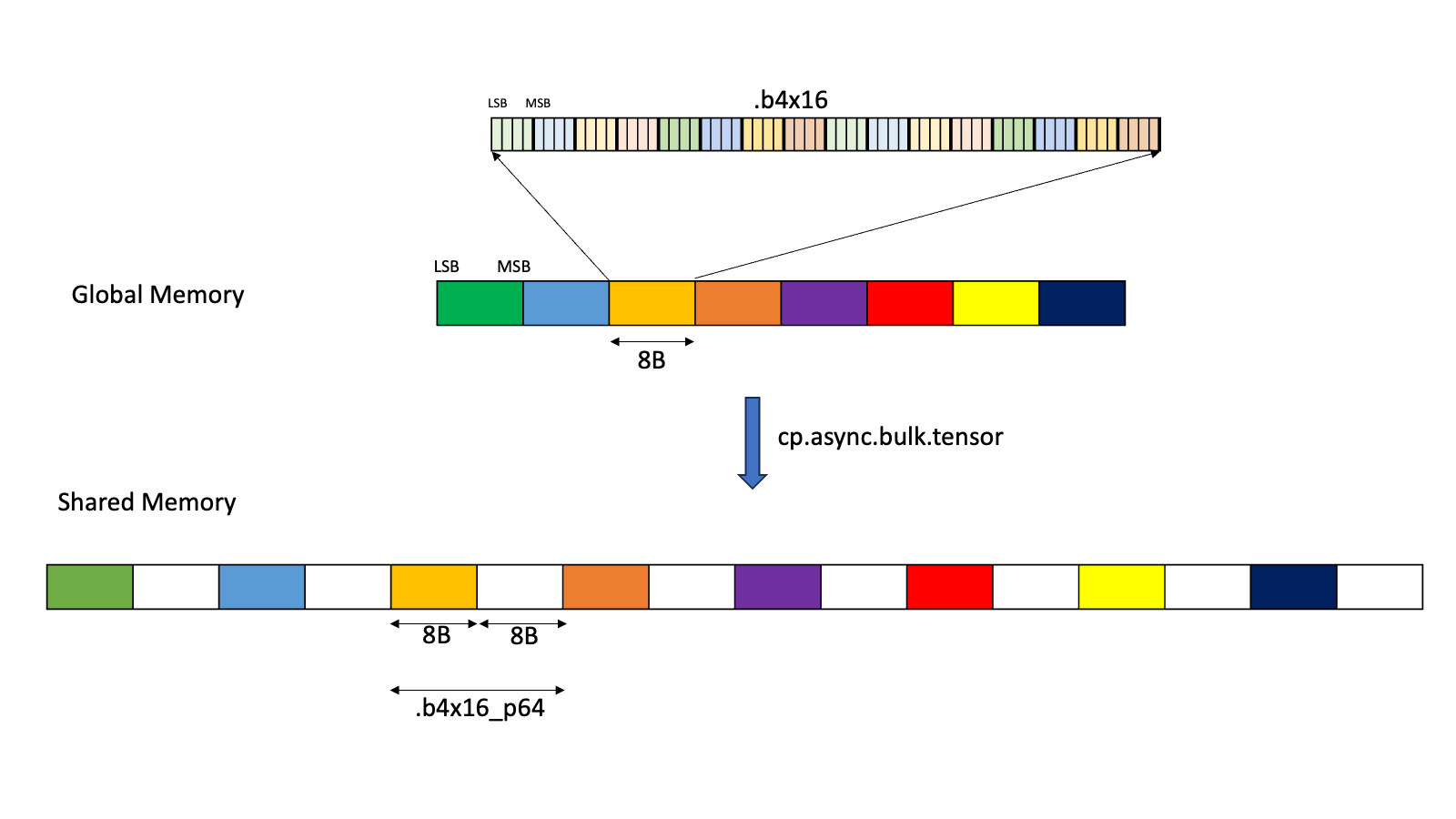
Figure 5 Layout for .b4x16_p64
The padded region that gets added is un-initialized.
-
Type
.b6x16_p32: With this type, sixteen 6-bits of data is copied from global memory to the shared memory with an append of 32-bits of padding as shown in Figure 6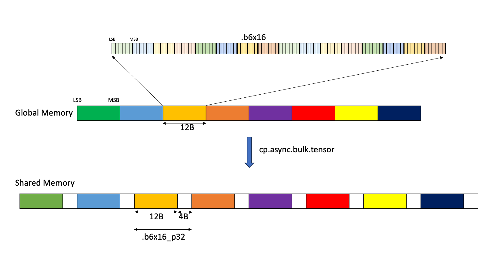
Figure 6 Layout for .b6x16_p32
The padded region that gets added is un-initialized.
-
Type
.b6p2x16: With this type, sixteen elements, each containing 6-bits of data at the LSB and 2-bits of padding at the MSB, are copied from shared memory into the global memory by discarding the 2-bits of padding data and packing the 6-bits data contiguously as shown in Figure 7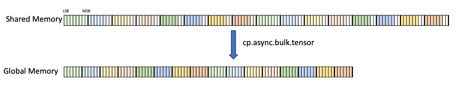
Figure 7 Layout for .b6p2x16
In case of .b6x16_p32 and .b4x16_p64, the padded region that gets added is
un-initialized.
The types .b6x16_p32 and .b6p2x16 share the same encoding value in the
descriptor (value 15) as the two types are applicable for different types of
tensor copy operations:
Type |
Valid Tensor Copy Direction |
|---|---|
|
|
|
|
5.5.2. Tensor Access Modes#
Tensor data can be accessed in two modes:
-
Tiled mode:
In tiled mode, the source multi-dimensional tensor layout is preserved at the destination.
-
Im2col mode:
In im2col mode, the elements in the Bounding Box of the source tensor are rearranged into columns at the destination. Refer here for more details.
5.5.3. Tiled Mode#
This section talks about how Tensor and Tensor access work in tiled mode.
5.5.3.1. Bounding Box#
A tensor can be accessed in chunks known as Bounding Box. The Bounding Box has the same dimensionality as the tensor they are accessing into. Size of each bounding Box must be a multiple of 16 bytes. The address of the bounding Box must also be aligned to 16 bytes.
Bounding Box has the following access properties:
Bounding Box dimension sizes
Out of boundary access mode
Traversal strides
The tensor-coordinates, specified in the PTX tensor instructions, specify the starting offset of the bounding box. Starting offset of the bounding box along with the rest of the bounding box information together are used to determine the elements which are to be accessed.
5.5.3.2. Traversal-Stride#
While the Bounding Box is iterating the tensor across a dimension, the traversal stride specifies the exact number of elements to be skipped. If no jump over is required, default value of 1 must be specified.
The traversal stride in dimension 0 can be used for the Interleave layout. For non-interleaved layout, the traversal stride in dimension 0 must always be 1.
Figure 8 illustrates tensor, tensor size, tensor stride, Bounding Box size and traversal stride.
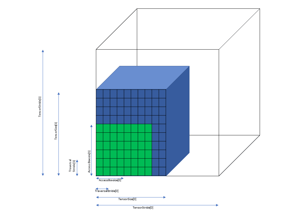
Figure 8 Tiled mode bounding box, tensor size and traversal stride
5.5.3.3. Out of Boundary Access#
PTX Tensor operation can detect and handle the case when the Bounding Box crosses the tensor boundary in any dimension. There are 2 modes:
-
Zero fill mode:
Elements in the Bounding Box which fall outside of the tensor boundary are set to 0.
-
OOB-NaNfill mode:Elements in the Bounding Box which fall outside of the tensor boundary are set to a special NaN called
OOB-NaN.
Figure 9 shows an example of the out of boundary access.
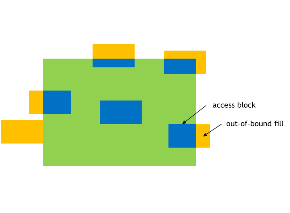
Figure 9 Out of boundary access
5.5.3.4. .tile::scatter4 and .tile::gather4 modes#
These modes are similar to the tiled mode with restriction that these modes work only on 2D tensor data.
Tile::scatter4 and Tile::gather4 modes are used to access multiple non-contiguous rows of tensor data.
In Tile::scatter4 mode single 2D source tensor is divided into four rows in the 2D destination tensor.
In Tile::gather4 mode four rows in the source 2D tensor are combined to form single 2D destination tensor.
These modes work on four rows and hence the instruction will take:
four tensor coordinates across the dimension 0
one tensor coordinate across the dimension 1
The interleave layout is not supported for .tile::scatter4 and .tile::gather4 modes.
All other constraints and rules of the tile mode apply to these modes as well.
5.5.3.4.1. Bounding Box#
For Tile::scatter4 and Tile::gather4 modes, four request coordinates will form four Bounding
Boxes in the tensor space.
Figure 10 shows an example of the same with start coordinates (1, 2), (1, 5), (1, 0) and (1, 9).
The size of the bounding box in the dimension 0 represents the length of the rows. The size of the bounding box in the dimension 1 must be one.
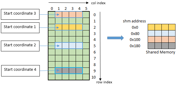
Figure 10 tiled::scatter4/tiled::gather4 mode bounding box example
5.5.4. im2col mode#
Im2col mode supports the following tensor dimensions : 3D, 4D and 5D. In this mode, the tensor data is treated as a batch of images with the following properties:
N : number of images in the batch
D, H, W : size of a 3D image (depth, height and width)
C: channels per image element
The above properties are associated with 3D, 4D and 5D tensors as follows:
Dimension |
N/D/H/W/C applicability |
|---|---|
3D |
NWC |
4D |
NHWC |
5D |
NDHWC |
5.5.4.1. Bounding Box#
In im2col mode, the Bounding Box is defined in DHW space. Boundaries along other dimensions are specified by Pixels-per-Column and Channels-per-Pixel parameters as described below.
The dimensionality of the Bounding Box is two less than the tensor dimensionality.
The following properties describe how to access of the elements in im2col mode:
Bounding-Box Lower-Corner
Bounding-Box Upper-Corner
Pixels-per-Column
Channels-per-Pixel
Bounding-box Lower-Corner and Bounding-box Upper-Corner specify the two opposite corners of the Bounding Box in the DHW space. Bounding-box Lower-Corner specifies the corner with the smallest coordinate and Bounding-box Upper-Corner specifies the corner with the largest coordinate.
Bounding-box Upper- and Lower-Corners are 16-bit signed values whose limits varies across the dimensions and are as shown below:
3D |
4D |
5D |
|
|---|---|---|---|
Upper- / Lower- Corner sizes |
[-215, 215-1] |
[-27, 27-1] |
[-24, 24-1] |
Figure 11 and Figure 12 show the Upper-Corners and Lower-Corners.
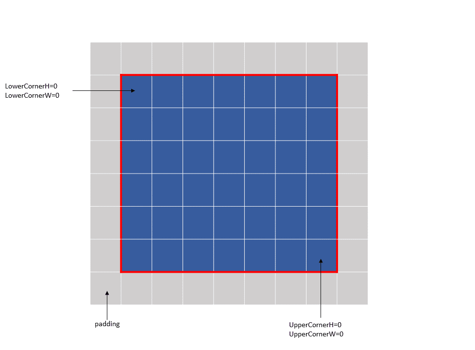
Figure 11 im2col mode bounding box example 1
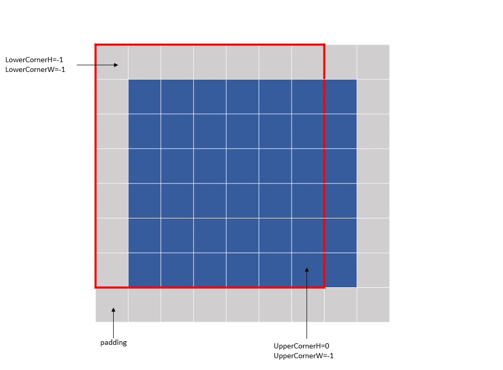
Figure 12 im2col mode bounding box example 2
The Bounding-box Upper- and Lower-Corners specify only the boundaries and not the number of elements to be accessed. Pixels-per-Column specifies the number of elements to be accessed in the NDHW space.
Channels-per-Pixel specifies the number of elements to access across the C dimension.
The tensor coordinates, specified in the PTX tensor instructions, behaves differently in different dimensions:
Across N and C dimensions: specify the starting offsets along the dimension, similar to the tiled mode.
Across DHW dimensions: specify the location of the convolution filter base in the tensor space. The filter corner location must be within the bounding box.
The im2col offsets, specified in the PTX tensor instructions in im2col mode, are added to the filter base coordinates to determine the starting location in the tensor space from where the elements are accessed.
The size of the im2col offsets varies across the dimensions and their valid ranges are as shown below:
3D |
4D |
5D |
|
|---|---|---|---|
im2col offsets range |
[0, 216-1] |
[0, 28-1] |
[0, 25-1] |
Following are some examples of the im2col mode accesses:
-
Example 1 (Figure 13):
Tensor Size[0] = 64
Tensor Size[1] = 9
Tensor Size[2] = 14
Tensor Size[3] = 64
Pixels-per-Column = 64
channels-per-pixel = 8
Bounding-Box Lower-Corner W = -1
Bounding-Box Lower-Corner H = -1
Bounding-Box Upper-Corner W = -1
Bounding-Box Upper-Corner H = -1.
tensor coordinates = (7, 7, 4, 0)
im2col offsets : (0, 0)
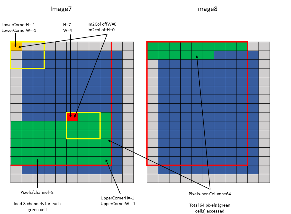
Figure 13 im2col mode example 1
-
Example 2 (Figure 14):
Tensor Size[0] = 64
Tensor Size[1] = 9
Tensor Size[2] = 14
Tensor Size[3] = 64
Pixels-per-Column = 64
channels-per-pixel = 8
Bounding-Box Lower-Corner W = 0
Bounding-Box Lower-Corner H = 0
Bounding-Box Upper-Corner W = -2
Bounding-Box Upper-Corner H = -2
tensor coordinates = (7, 7, 4, 0)
im2col offsets: (2, 2)
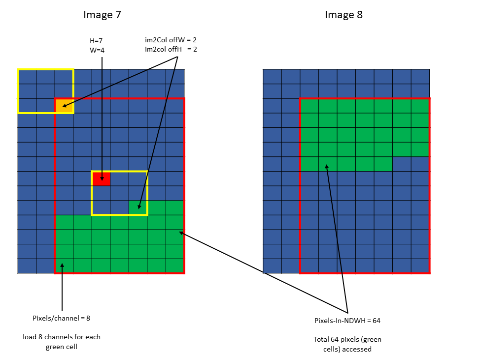
Figure 14 im2col mode example 2
5.5.4.2. Traversal Stride#
The traversal stride, in im2col mode, does not impact the total number of elements (or pixels) being accessed unlike the tiled mode. Pixels-per-Column determines the total number of elements being accessed, in im2col mode.
The number of elements traversed along the D, H and W dimensions is strided by the traversal stride for that dimension.
The following example with Figure 15 illustrates accesses with traversal-strides:
Tensor Size[0] = 64
Tensor Size[1] = 8
Tensor Size[2] = 14
Tensor Size[3] = 64
Traversal Stride = 2
Pixels-per-Column = 32
channels-per-pixel = 16
Bounding-Box Lower-Corner W = -1
Bounding-Box Lower-Corner H = -1
Bounding-Box Upper-Corner W = -1
Bounding-Box Upper-Corner H = -1.
Tensor coordinates in the instruction = (7, 7, 5, 0)
Im2col offsets in the instruction : (1, 1)
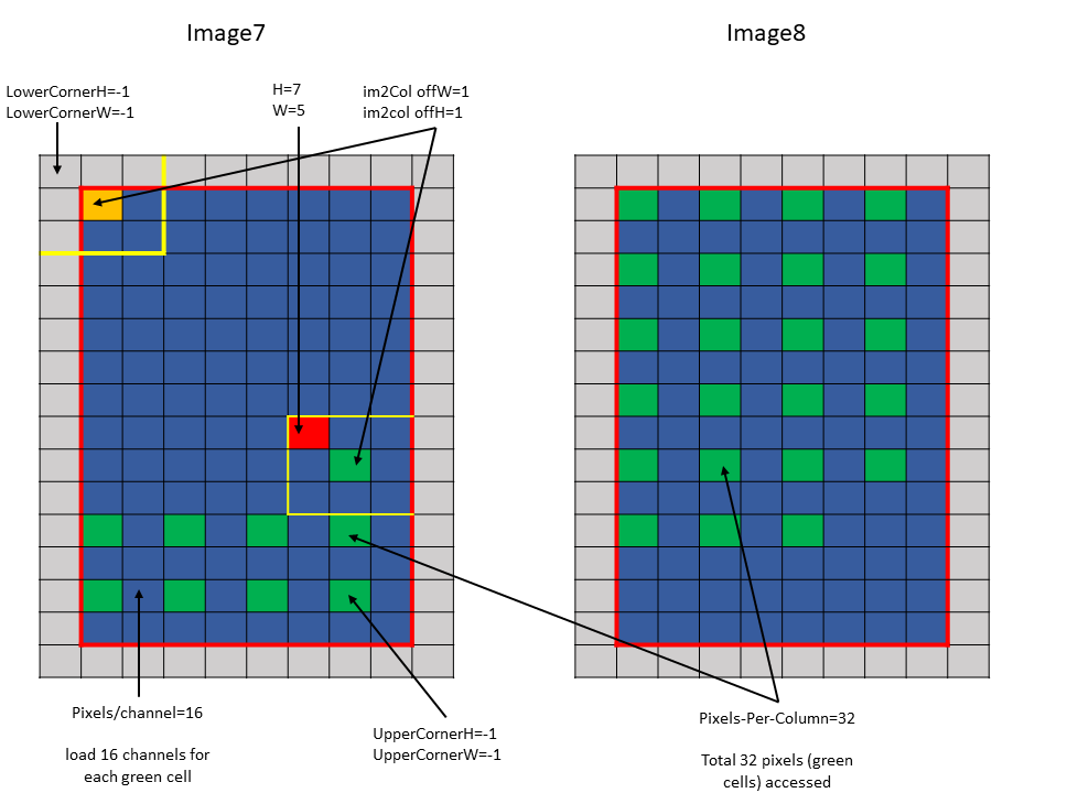
Figure 15 im2col mode traversal stride example
5.5.4.3. Out of Boundary Access#
In im2col mode, when the number of requested pixels in NDHW space specified by Pixels-per-Column exceeds the number of available pixels in the image batch then out-of-bounds access is performed.
Similar to tiled mode, zero fill or OOB-NaN fill can be performed based on the Fill-Mode
specified.
5.5.5. im2col::w , im2col_no_offs::w and im2col::w::128 modes#
These modes are similar to the im2col mode with the restriction that elements are accessed across
the W dimension only while keeping the H and D dimension constant.
All the constraints and rules of the im2col mode apply to these modes as well. Note that for these modes, the legal Swizzling Modes is required. In other words, swizzling mode must not be set to (i) no swizzle and (ii) 128-byte swizzle mode with 32-byte atomicity with 8-byte flip.
The number of elements accessed in the im2col::w::128 mode is fixed and is equal to 128.
The number of elements accessed in the im2col::w and im2col_no_offs::w modes depend on the
Pixels-per-Column field in the TensorMap.
5.5.5.1. Bounding Box#
In these modes, the size of the bounding box in D and H dimensions are 1.
The D and H dimensions in the tensor coordinates argument in the PTX instruction specify
the position of the bounding box in the tensor space.
The Bounding-Box Lower-Corner-W and Bounding-Box Upper-Corner-W specify the two opposite
corners of the Bounding Box in the W dimension.
The W dimension in the tensor coordinates argument in the PTX instruction specify the location
of the first element that is to be accessed in the bounding box.
Number of pixels loaded in im2col::w mode and number of pixels stored or otherwise reduced in
im2col_no_offs::w mode is specified by Pixels-per-Column in the TensorMap.
Number of pixels loaded in im2col::w::128 mode is always 128. So, Pixels-per-Column is ignored
in im2col::w::128 mode.
Figure 16 shows an example of the im2col::w and
im2col::w:128 modes.
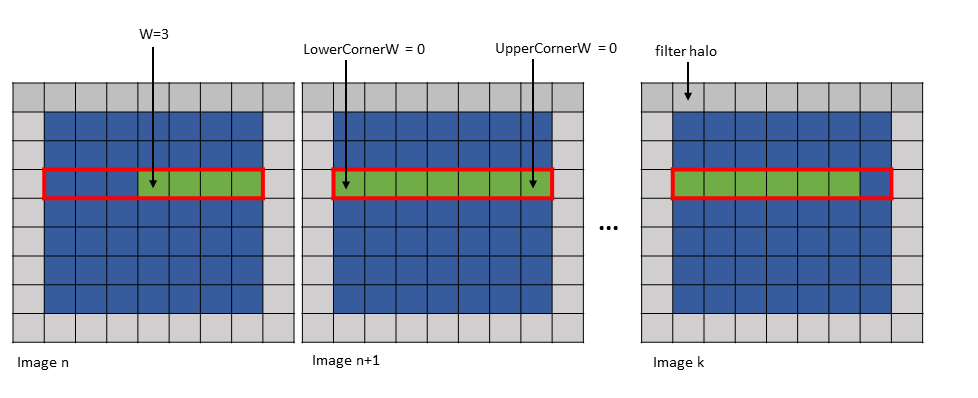
Figure 16 im2col::w and im2col::w::128 modes example
The first element can lie outside of the Bounding Box in the W-dimension only and only on the left side of the Bounding Box. Figure 17 shows of an example of this.
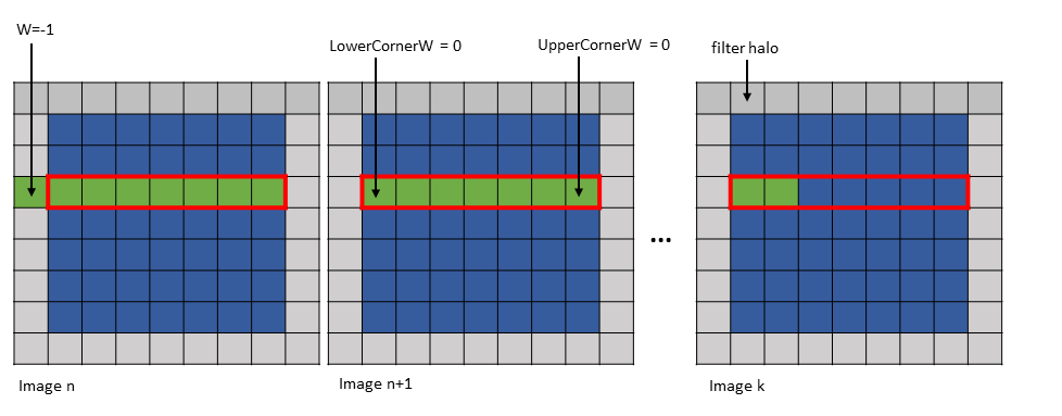
Figure 17 im2col::w and im2col::w::128 modes first element outside Bounding Box example
For im2col_no_offs::w mode, since the tensor data is being stored or otherwise reduced to global memory,
the bounding box must always stay within the tensor boundary limit. In other words, the numeric value for
Lower-Corner-W must be non-negative while the value for Upper-Corner-W must be non-positive. In this mode,
it also naturally follows that the negative values for tensor coordinates would result in illegal out-of-bounds
access and runtime error is raised in such cases.
Additionally, note that once out of boundary access is detected, subsequent pixel operations would not be
performed even if the total count of the pixel operated is less than the Pixels-per-Column value specified
in the TensorMap.
Figure 18 shows an example of the im2col_no_offs::w mode.
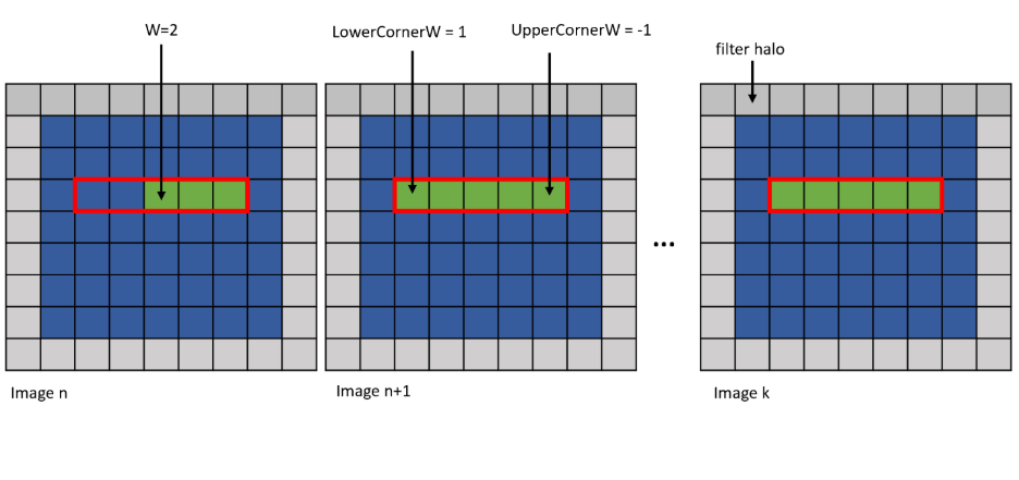
Figure 18 im2col_no_offs::w mode example
5.5.5.2. Traversal Stride#
This is similar to im2col mode with the exception of that the number of elements traversed
along only the W dimension is strided by the traversal stride as specified in the TensorMap.
5.5.5.3. wHalo#
In im2col::w mode, the wHalo argument in the PTX instruction specifies how many filter
halo elements must be loaded at the end of the image.
In im2col::w::128 mode, the halo elements are loaded after every 32 elements in the bounding
box along the W dimension. The wHalo argument in the PTX instruction specifies how many
halo elements must be loaded after every 32 elements.
Note that for im2col_no_offs::w mode, it is illegal to explicitly specify wHalo value and
instead it always defaults to 0.
Following is an example of .im2col::w mode access:
Tensor Size [0] = 128
Tensor Size [1] = 9
Tensor Size [2] = 7
Tensor Size [3] = 64
Pixels-per-column = 128
Channels-per-pixel = 64
Bounding Box Lower Corner W = 0
Bounding Box Upper Corner W = 0
Tensor Coordinates in the instruction = (7, 2, 3, 0)
wHalo in the instruction = 2 (as 3x3 convolution filter is used)
A tensor copy operation with the above parameters loads 128 pixels and the two halo pixels as shown in Figure 19.
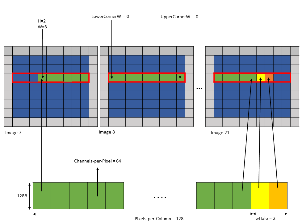
Figure 19 tensor copy operation with im2col::w mode example
The halo pixels are always loaded in the shared memory next to the main row pixels as shown in Figure 19.
Following is an example of .im2col::w::128 mode access:
Tensor Size [0] = 128
Tensor Size [1] = 9
Tensor Size [2] = 7
Tensor Size [3] = 64
Channels-per-pixel = 64
Bounding Box Lower Corner W = 0
Bounding Box Upper Corner W = 0
Tensor Coordinates in the instruction = (7, 2, 3, 0)
wHalo in the instruction = 2 (as 3x3 convolution filter is used)
A tensor copy operation with the above parameters loads 128 elements such that after every 32 elements, wHalo number of elements are loaded as shown in Figure 20.
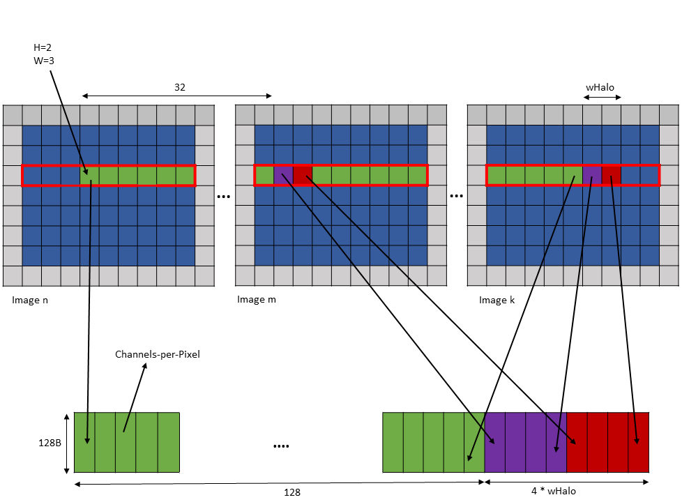
Figure 20 tensor copy operation with im2col::w::128 mode example
5.5.5.4. wOffset#
In the convolution calculations, the same elements along the W dimension are reused for different
locations within the convolution filter footprint. Based on the number of times a pixel is used, the
pixels may be loaded into different shared memory buffers. Each buffer can be loaded by a separate
tensor copy operation.
The wOffset argument in the tensor copy and prefetch instruction adjusts the source pixel location
for each buffer. The exact position of the buffer is adjusted along the W dimension using the
following formula:
Bounding Box Lower Corner W += wOffset
Bounding Box Upper Corner W += wOffset
W += wOffset
Note that for im2col_no_offs::w mode, it is illegal to explicitly specify wOffset value and
instead it always defaults to 0.
Following are examples of tensor copy to multiple buffers with various wHalo and wOffset values:
Example 1:
Tensor Size [0] = 128
Tensor Size [1] = 9
Tensor Size [2] = 67
Tensor Size [3] = 64
Pixels-per-Column = 128
Channels-per-pixel = 64
Bounding Box Lower Corner W = -1
Bounding Box Upper Corner W = 0
Traversal Stride = 2
Tensor Coordinates in the instruction = (7, 2, -1, 0)
Shared memory buffer 1:
wHalo = 1
wOffset = 0
Shared memory buffer 2:
wHalo = 0
wOffset = 1
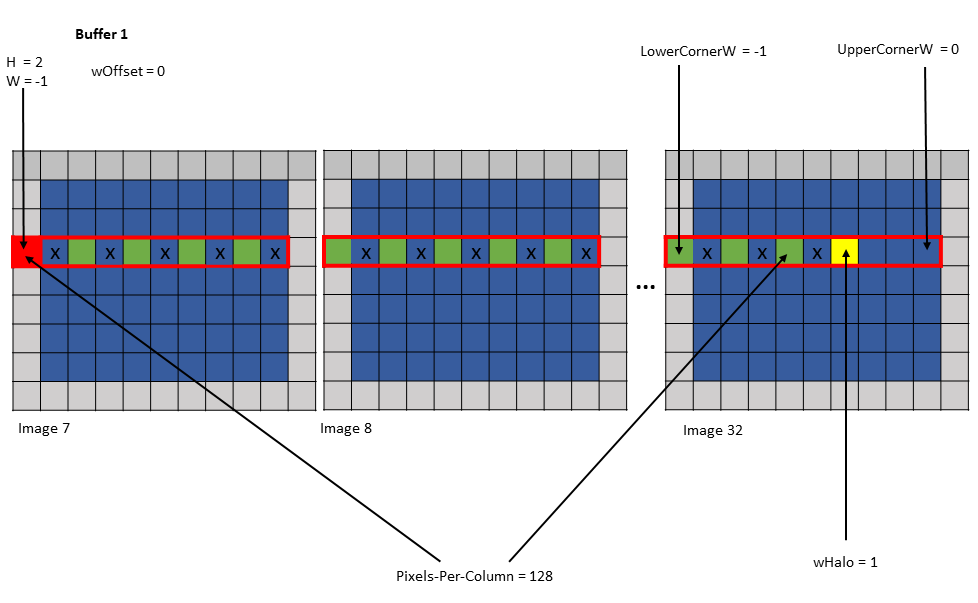
Figure 21 tensor copy operation to buffer 1 of Example 1
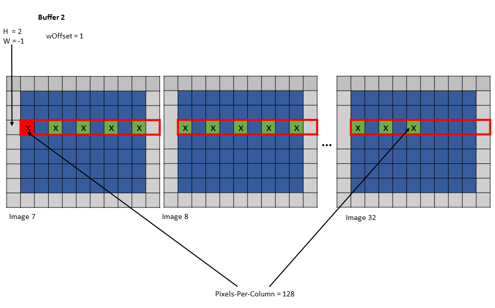
Figure 22 tensor copy operation to buffer 2 of Example 1
Example 2:
Tensor Size [0] = 128
Tensor Size [1] = 7
Tensor Size [2] = 7
Tensor Size [3] = 64
Pixels-per-Column = 128
Channels-per-pixel = 64
Bounding Box Lower Corner W = -1
Bounding Box Upper Corner W = -1
Traversal Stride = 3
Tensor Coordinates in the instruction = (7, 2, -1, 0)
Shared memory buffer 1:
wHalo = 0
wOffset = 0
Shared memory buffer 2:
wHalo = 0
wOffset = 1
Shared memory buffer 3:
wHalo = 0
wOffset = 2
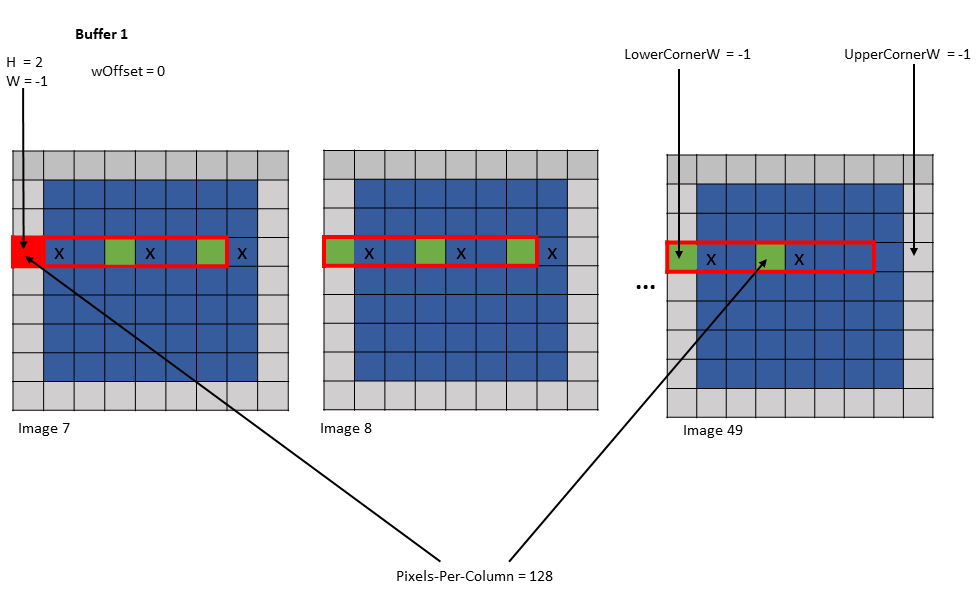
Figure 23 tensor copy operation to buffer 1 of Example 2
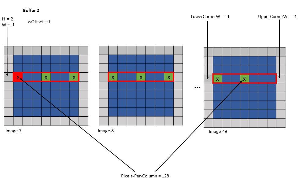
Figure 24 tensor copy operation to buffer 2 of Example 2
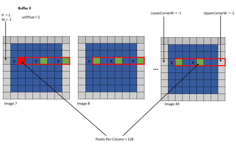
Figure 25 tensor copy operation to buffer 3 of Example 2
5.5.6. Interleave layout#
Tensor can be interleaved and the following interleave layouts are supported:
No interleave (NDHWC)
8 byte interleave (NC/8DHWC8) : C8 utilizes 16 bytes in memory assuming 2B per channel.
16 byte interleave (NC/16HWC16) : C16 utilizes 32 bytes in memory assuming 4B per channel.
The C information is organized in slices where sequential C elements are grouped in 16 byte or 32 byte quantities.
If the total number of channels is not a multiple of the number of channels per slice, then the last slice must be padded with zeros to make it complete 16B or 32B slice.
Interleaved layouts are supported only for the dimensionalities : 3D, 4D and 5D.
The interleave layout is not supported for .im2col::w and .im2col::w::128 modes.
5.5.7. Swizzling Modes#
The layout of the data in the shared memory can be different to that of global memory, for access performance reasons. The following describes various swizzling modes:
-
No swizzle mode:
There is no swizzling in this mode and the destination data layout is exactly similar to the source data layout.
0
1
2
3
4
5
6
7
0
1
2
3
4
5
6
7
… Pattern repeats …
-
32 byte swizzle mode:
The following table, where each elements (numbered cell) is 16 byte and the starting address is 256 bytes aligned, shows the pattern of the destination data layout:
0
1
2
3
4
5
6
7
1
0
3
2
5
4
7
6
… Pattern repeats …
An example of the 32 byte swizzle mode for NC/(32B)HWC(32B) tensor of 1x2x10x10xC16 dimension, with the innermost dimension holding slice of 16 channels with 2 byte/channel, is shown in Figure 26.
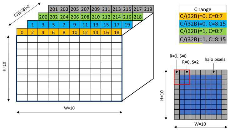
Figure 26 32-byte swizzle mode example
Figure 27 shows the two fragments of the tensor : one for C/(32B) = 0 and another for C/(32B) = 1.
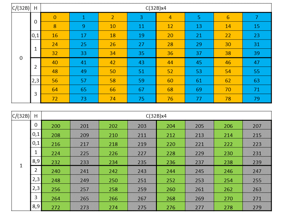
Figure 27 32-byte swizzle mode fragments
Figure 28 shows the destination data layout with 32 byte swizzling.
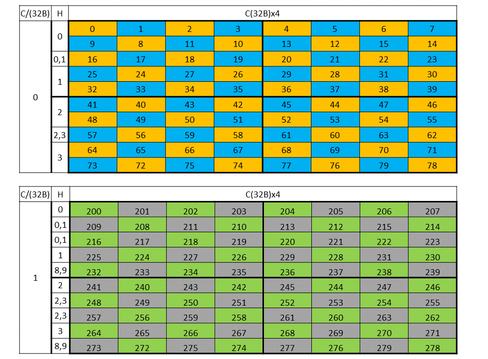
Figure 28 32-byte swizzle mode destination data layout
-
64 byte swizzle mode:
The following table, where each elements (numbered cell) is 16 byte and the starting address is 512 bytes aligned, shows the pattern of the destination data layout:
0
1
2
3
4
5
6
7
1
0
3
2
5
4
7
6
2
3
0
1
6
7
4
5
3
2
1
0
7
6
5
4
… Pattern repeats …
An example of the 64 byte swizzle mode for NHWC tensor of 1x10x10x64 dimension, with 2 bytes / channel and 32 channels, is shown in Figure 29.
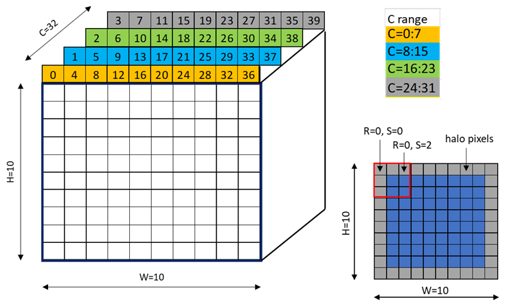
Figure 29 64-byte swizzle mode example
Each colored cell represents 8 channels. Figure 30 shows the source data layout.
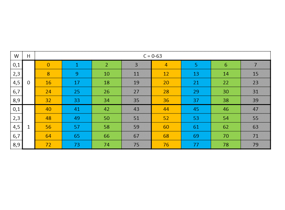
Figure 30 64-byte swizzle mode source data layout
Figure 31 shows the destination data layout with 64 byte swizzling.
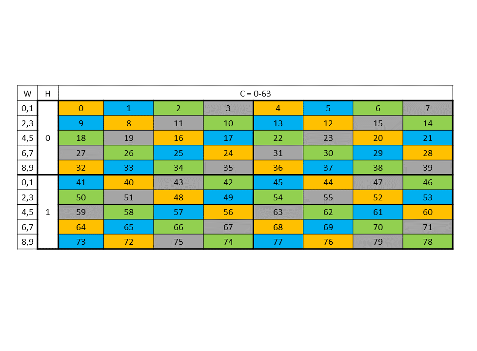
Figure 31 64-byte swizzle mode destination data layout
-
96 byte swizzle mode:
The following table where each element (numbered cell) is 16 byte shows the swizzling pattern at the destination data layout:
0
1
2
3
4
5
6
7
1
0
3
2
5
4
7
6
… Pattern repeats …
An example of the data layout in global memory and its swizzled data layout in shared memory where each element (colored cell) is 16 bytes and the starting address is 256 bytes aligned is shown in Figure 32.
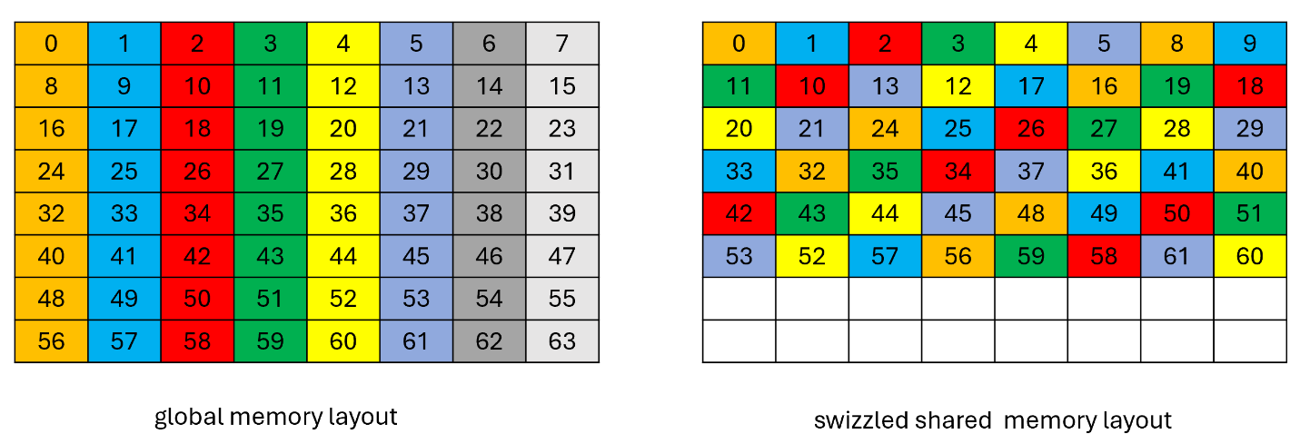
Figure 32 96-byte swizzle mode example
-
128 byte swizzle mode:
The 128-byte swizzling mode supports the following sub-modes:
-
16-byte atomicity sub-mode:
In this sub-mode, the 16-byte of data is kept intact while swizzling.
The following table, where each elements (numbered cell) is 16 byte and the starting address is 1024 bytes aligned, shows the pattern of the destination data layout:
0
1
2
3
4
5
6
7
1
0
3
2
5
4
7
6
2
3
0
1
6
7
4
5
3
2
1
0
7
6
5
4
4
5
6
7
0
1
2
3
5
4
7
6
1
0
3
2
6
7
4
5
2
3
0
1
7
6
5
4
3
2
1
0
… Pattern repeats …
An example of the 128 byte swizzle mode for NHWC tensor of 1x10x10x64 dimension, with 2 bytes / channel and 64 channels, is shown in Figure 33.
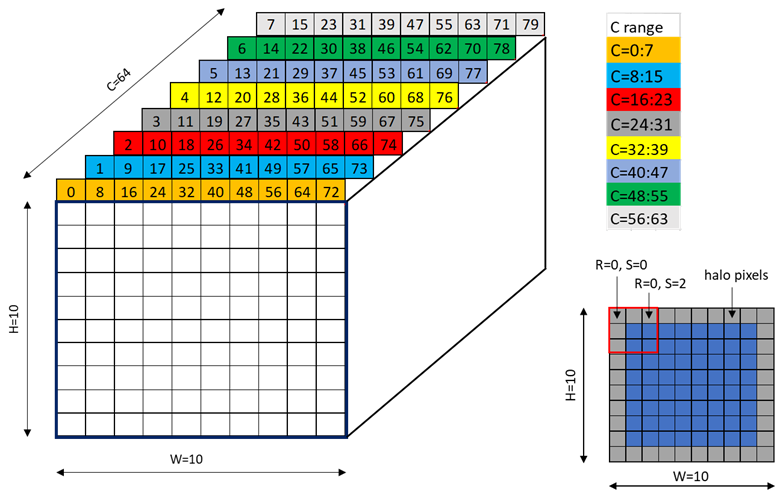
Figure 33 128-byte swizzle mode example
Each colored cell represents 8 channels. Figure 34 shows the source data layout.
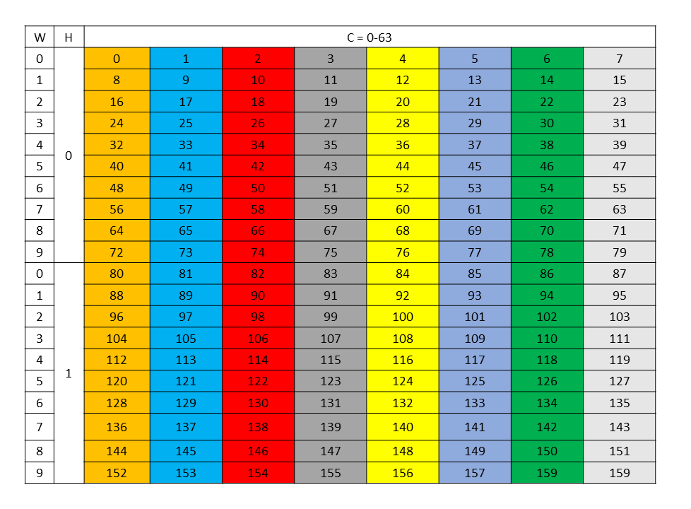
Figure 34 128-byte swizzle mode source data layout
Figure 35 shows the destination data layout with 128 byte swizzling.
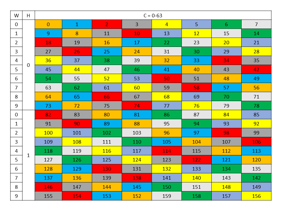
Figure 35 128-byte swizzle mode destination data layout
-
32-byte atomicity sub-mode:
In this sub-mode, the 32-byte of data is kept intact while swizzling.
The following table where each element (numbered cell) is 16 byte shows the swizzling pattern at the destination data layout:
0 1
2 3
4 5
6 7
2 3
0 1
6 7
4 5
4 5
6 7
0 1
2 3
6 7
4 5
2 3
0 1
… Pattern repeats …
This sub-mode requires 32 byte alignment at shared memory.
An example of the data layout in global memory and its swizzled data layout in shared memory where each element (colored cell) is 16 bytes is shown in Figure 36
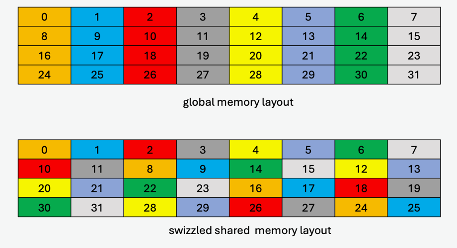
Figure 36 128-byte swizzle mode example with 32-byte atomicity
-
32-byte atomicity with 8-byte flip sub-mode:
The swizzling pattern for this sub-mode is similar to the 32-byte atomicity sub-mode except that there is a flip of adjacent 8-bytes within the 16-byte data at every alternate shared memory line. Note that this mode is legal only when
cp.async.bulk.tensorspecifies the copy direction as.shared::cluster.globalor otherwise.shared::cta.global.An example of the data layout in global memory and its swizzled data layout in shared memory where each element (colored cell) is 16 bytes (two 8-byte sub-elements for each 16-byte colored cell are shown to show the flip) is shown in Figure 37
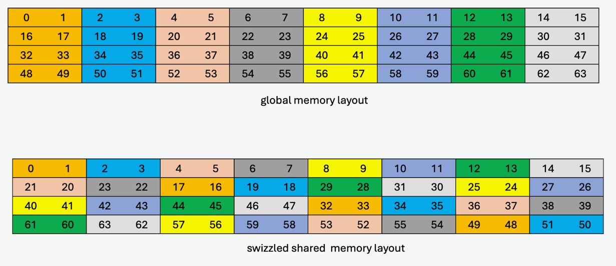
Figure 37 128-byte swizzle mode example with 32-byte atomicity with 8-byte flip
-
64-byte atomicity sub-mode:
In this sub-mode, the 64-byte of data is kept intact while swizzling.
The following table where each element (numbered cell) is 16 byte shows the swizzling pattern at the destination data layout:
0 1 2 3
4 5 6 7
4 5 6 7
0 1 2 3
… Pattern repeats …
This sub-mode requires 64-byte alignment at shared memory.
An example of the data layout in global memory and its swizzled data layout in shared memory where each element (colored cell) is 16 bytes is shown in Figure 38
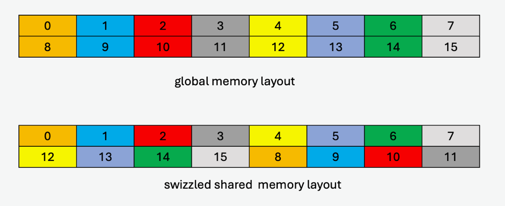
Figure 38 128-byte swizzle mode example with 64-byte atomicity
-
Table 14 lists the valid combination of swizzle-atomicity with the swizzling-mode.
Swizzling Mode |
Swizzle-Atomicity |
|---|---|
No Swizzling |
– |
32B Swizzling Mode |
16B |
64B Swizzling Mode |
16B |
96B Swizzling Mode |
16B |
128B Swizzling Mode |
|
The value of swizzle base offset is 0 when the dstMem shared memory address is located
at the following boundary:
Swizzling Mode |
Starting address of the repeating pattern |
|---|---|
128-Byte swizzle |
1024-Byte boundary |
96-Byte swizzle |
256-Byte boundary |
64-Byte swizzle |
512-Byte boundary |
32-Byte swizzle |
256-Byte boundary |
Otherwise, the swizzle base offset is a non-zero value, computed using following formula:
Swizzling Mode |
Formula |
|---|---|
128-Byte swizzle |
base offset = (dstMem / 128) % 8 |
96-Byte swizzle |
base offset = (dstMem / 128) % 2 |
64-Byte swizzle |
base offset = (dstMem / 128) % 4 |
32-Byte swizzle |
base offset = (dstMem / 128) % 2 |
5.5.8. Tensor-map#
The tensor-map is a 128-byte opaque object either in .const space or .param (kernel function
parameter) space or .global space which describes the tensor properties and the access properties
of the tensor data described in previous sections.
Tensor-Map can be created using CUDA APIs. Refer to CUDA programming guide for more details.